This blog is written as a supplementary for this practical guide to diffusion models (Elflein, 2022), which I think is an excellent material for diffusion learning.
Diffusion
Diffusion models define a forward and backward process:
- the forward process gradually adds noise to the data until the original data is indistinguishable (one arrives at a standard normal distribution $N(0, \mathbf{I})$)
- the backward process aims to reverse the forward process, i.e., start from noise and then gradually tries to restore data
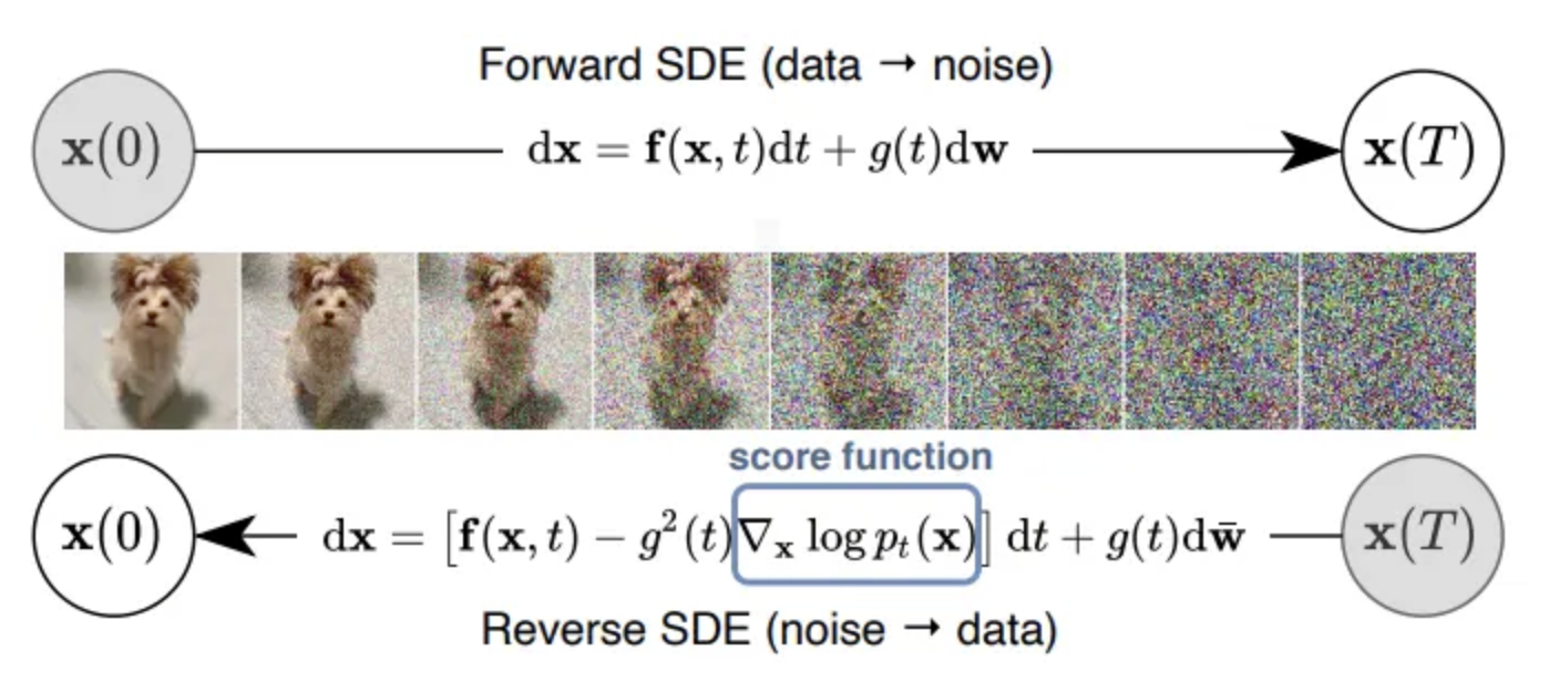
To generate new samples by starting from random noise, one aims to learn the backward process.
To be able to start training a model that learns this backward process, we first need to know how to do the forward process.
Forward
The forward process adds noise at every step $t$ controlled by parameters \(\{\alpha_t\}_{t=1, \dots, T}, \alpha_{t-1} > \alpha_t, \alpha_T = 0\):
\[\begin{equation} q(x_t \mid x_{t-1}) \sim \mathcal{N}(\sqrt{\alpha_t}x_{t-1}, (1-\alpha_t)\mathbf{I}) \end{equation}\]As \(t \rightarrow T\) this distribution becomes a multi-variate Gaussian distribution \(\mathcal{N}(0, \mathbf{I})\).
So why do we include a $\alpha$ here? Why can’t we just add standard noise every single time? Wouldn’t that make things simpler? No. Intuitively, think about it this way: when you add noise to a clean image, even a small amount initially has a visible blurring effect. However, as the image becomes increasingly noisy, you have to add significantly more noise to make any perceptible difference. From a mathematical perspective, the denoising process requires this specific noise intensity (schedule) to ensure the distance function remains differentiable. For more specific details, you can refer to the materials linked above (e.g. Yuan et al., 2024).
The cool thing about this being Gaussian noise is that instead of simulating this forward process by iteratively sampling noise, one can derive a closed form for the distribution at a certain $t$ given the original data point $x_0$ so one has to only sample noise once:
\[\begin{equation} q(x_t \mid x_0) \sim \mathcal{N}(\sqrt{\bar{\alpha}}_t x_0, (1 - \bar{\alpha}_t)\mathbf{I}) \end{equation}\]with $\bar{\alpha}_t = \prod_{s = 1}^t \alpha_s$.
How do we get this formula?
We know that \(x_1 = \sqrt{\alpha_1} x_0 + \sqrt{1 - \alpha_1} \epsilon_0\) and \(x_2 = \sqrt{\alpha_2} x_1 + \sqrt{1 - \alpha_2} \epsilon_1\)
so \(x_2 = \sqrt{\alpha_2} (\sqrt{\alpha_1} x_0 + \sqrt{1 - \alpha_1} \epsilon_0) + \sqrt{1 - \alpha_2} \epsilon_1\)
then \(x_2 = \sqrt{\alpha_1 \alpha_2} x_0 + \sqrt{\alpha_2 (1 - \alpha_1)} \epsilon_0 + \sqrt{1 - \alpha_2} \epsilon_1\)
Note that:
- Term A: $\sqrt{\alpha_2 (1 - \alpha_1)} \epsilon_0 \sim \mathcal{N}(0, \alpha_2(1-\alpha_1)\mathbf{I})$
- Term B: $\sqrt{1 - \alpha_2} \epsilon_1 \sim \mathcal{N}(0, (1-\alpha_2)\mathbf{I})$
Since $\epsilon_0$ and $\epsilon_1$ are independent, their sum still follows a Gaussian distribution. The total variance is equal to the sum of their individual variances:
\[\sigma^2_{total} = \alpha_2(1-\alpha_1) + (1-\alpha_2)\] \[\sigma^2_{total} = \alpha_2 - \alpha_1\alpha_2 + 1 - \alpha_2 = 1 - \alpha_1\alpha_2\]By defining $\bar{\alpha}_2 = \alpha_1 \alpha_2$, we can merge these two noise terms into a single new standard Gaussian noise $\bar{\epsilon}_2$:
\[x_2 = \sqrt{\bar{\alpha}_2} x_0 + \sqrt{1 - \bar{\alpha}_2} \bar{\epsilon}_2\]Hope you get some insight to calculate $x_n$.
Training
Next, we want to train a model that reverses that process.
For this, one can show that the there is also a closed form for the less noisy version $x_{t-1}$ given the next sample $x_t$ and the original sample $x_0$.
\[\begin{equation} q(x_{t-1} \mid x_t, x_0) = \mathcal{N}(\mu(x_t, x_0), \sigma_t^2\mathbf{I}) \end{equation}\]where
\[\begin{equation} \sigma_t^2 = \frac{(1 - \alpha_t)(1 - \bar{\alpha}_{t-1})}{1 - \bar{\alpha}_t}, \quad \mu(x_t, x_0) = \frac{1}{\sqrt{\alpha_t}} \left(x_t - \frac{1 - \alpha_t}{\sqrt{1 - \bar{\alpha}_t}} \epsilon_0\right) \end{equation}\]and $\epsilon_0 \sim \mathcal{N}(0, \mathbf{I})$ is the noise drawn to perturb the original data $x_0$.
Why? Please don’t be overwhelmed by the following. Based on Bayes’ rule, we can express $q(x_{t-1} | x_t, x_0)$ as:
\[q(x_{t-1} | x_t, x_0) = q(x_t | x_{t-1}, x_0) \frac{q(x_{t-1} | x_0)}{q(x_t | x_0)}\]Since the diffusion process is a Markov chain, once $x_{t-1}$ is given, the distribution of $x_t$ becomes independent of $x_0$. Therefore, \(q(x_t | x_{t-1}, x_0) = q(x_t | x_{t-1})\). The formula simplifies to:
\[q(x_{t-1} | x_t, x_0) = q(x_t | x_{t-1}) \frac{q(x_{t-1} | x_0)}{q(x_t | x_0)}\]During the forward process, we have already defined or derived the three terms on the right-hand side:
-
Single-step forward: \(q(x_t | x_{t-1}) = \mathcal{N}(x_t; \sqrt{\alpha_t} x_{t-1}, (1-\alpha_t) \mathbf{I})\)
-
Direct mapping to $t-1$: \(q(x_{t-1} | x_0) = \mathcal{N}(x_{t-1}; \sqrt{\bar{\alpha}_{t-1}} x_0, (1-\bar{\alpha}_{t-1}) \mathbf{I})\)
-
Direct mapping to $t$: \(q(x_t | x_0) = \mathcal{N}(x_t; \sqrt{\bar{\alpha}_t} x_0, (1-\bar{\alpha}_t) \mathbf{I})\)
Since the product or division of Gaussian distributions remains Gaussian, we only need to focus on the terms inside the exponential $\exp(-\frac{1}{2}(\dots))$.
Substituting the three distributions above into Bayes’ rule, the exponential part (ignoring the $-1/2$ factor) expands to:
\[\frac{(x_t - \sqrt{\alpha_t} x_{t-1})^2}{1-\alpha_t} + \frac{(x_{t-1} - \sqrt{\bar{\alpha}_{t-1}} x_0)^2}{1-\bar{\alpha}_{t-1}} - \frac{(x_t - \sqrt{\bar{\alpha}_t} x_0)^2}{1-\bar{\alpha}_t}\]Because we are solving for the distribution of $x_{t-1}$, we need to rearrange this expression into the standard form $\frac{(x_{t-1} - \mu)^2}{\sigma^2}$ by completing the square.
Extracting the Variance $\sigma_t^2$
By isolating all terms involving $x_{t-1}^2$, the coefficient is:
\[\frac{\alpha_t}{1-\alpha_t} + \frac{1}{1-\bar{\alpha}_{t-1}} = \frac{\alpha_t(1-\bar{\alpha}_{t-1}) + 1 - \alpha_t}{(1-\alpha_t)(1-\bar{\alpha}_{t-1})} = \frac{1 - \bar{\alpha}_t}{(1-\alpha_t)(1-\bar{\alpha}_{t-1})}\]Taking the reciprocal of this coefficient gives us the variance formula:
\[\sigma_t^2 = \frac{(1-\alpha_t)(1-\bar{\alpha}_{t-1})}{1-\bar{\alpha}_t}\]Extracting the Mean $\mu(x_t, x_0)$
Similarly, by extracting and simplifying all terms containing $x_{t-1}$, we obtain:
\[\mu(x_t, x_0) = \frac{\sqrt{\alpha_t}(1-\bar{\alpha}_{t-1})}{1-\bar{\alpha}_t} x_t + \frac{\sqrt{\bar{\alpha}_{t-1}}(1-\alpha_t)}{1-\bar{\alpha}_t} x_0\]Introducing $\epsilon_0$ for Reparameterization
This is the final and most ingenious step. To enable the model to predict only the noise $\epsilon$, we utilize the forward process formula:
\[x_t = \sqrt{\bar{\alpha}_t} x_0 + \sqrt{1-\bar{\alpha}_t} \epsilon_0 \implies x_0 = \frac{1}{\sqrt{\bar{\alpha}_t}}(x_t - \sqrt{1-\bar{\alpha}_t} \epsilon_0)\]Substituting this expression for $x_0$ into the mean formula $\mu$ and performing some algebraic simplification (using the identity \(\bar{\alpha}_t = \alpha_t \bar{\alpha}_{t-1}\)), we arrive at the final form:
\[\mu(x_t, x_0) = \frac{1}{\sqrt{\alpha_t}} \left( x_t - \frac{1-\alpha_t}{\sqrt{1-\bar{\alpha}_t}} \epsilon_0 \right)\]Inference
After training the model to predict the noise $\epsilon$, we can simply iteratively run the backward process to predict $\mathbf{x}_{t-1}$ from $x_t$ starting from random noise $\mathbf{x}_T \sim \mathcal{N}(0, \mathbf{I})$.
\[\begin{equation} \mu(x_t) = \frac{1}{\sqrt{\alpha_t}} \left(x_t - \frac{1 - \alpha_t}{\sqrt{1 - \bar{\alpha}_t}} \epsilon_{\mathbf{\theta}}(\mathbf{x}_t, t) \right) \end{equation}\]One can see that as $t \rightarrow 0$ more fine-grained structure emerges that guides the sample to the original data manifold. At $t=T$ samples are guided coarsely towards the center as the signal is still very noisy and hard for the network to predict. This is further shown in Luo et al. (2022).
If you are interested in a more mathematical description with proofs I can highly recommend Luo et al. (2022).
Good Materials
See the linked practical guide and the references mentioned in the text above for full citations.